42 rotate data labels excel chart
Rotate DataLables in Excel chart Series The Tick Mark orientation can be changed to any angle from 0 to 90 degrees. This is the VBA code I got. VBnet should be the same except you don't use the word SET in the instructions. Set ChartObj = Sheets ("sheet1").ChartObjects ("Chart 1") Set oChart = ChartObj.Chart Set xAxis = oChart.Axes (xlCategory) With xAxis.TickLabels › documents › excelHow to rotate axis labels in chart in Excel? - ExtendOffice Rotate axis labels in Excel 2007/2010. 1. Right click at the axis you want to rotate its labels, select Format Axis from the context menu. See screenshot: 2. In the Format Axis dialog, click Alignment tab and go to the Text Layout section to select the direction you need from the list box of Text direction. See screenshot: 3.
exceljet.net › lessons › how-to-reverse-a-chart-axisExcel tutorial: How to reverse a chart axis Let me insert a standard column chart and let's look at how Excel plots the data. When Excel plots data in a column chart, the labels run from left to right to left. In this case, the first column is Cuba, and the last is Barbados, so the columns match the order of the source data moving moving top to bottom.

Rotate data labels excel chart
› charts › add-data-pointAdd Data Points to Existing Chart – Excel & Google Sheets Similar to Excel, create a line graph based on the first two columns (Months & Items Sold) Right click on graph; Select Data Range . 3. Select Add Series. 4. Click box for Select a Data Range. 5. Highlight new column and click OK. Final Graph with Single Data Point How to Rotate Pie Chart in Excel? - WallStreetMojo To rotate the pie chart, click on the chart area. Right-click on the pie chart and select the "format data series" option. Change the angle of the first scale to 90 degrees to display the chart properly. Now the pie chart is looking good, representing clearly the small slices. Example #2 - 3D Rotate Pie Chart Rotate a Chart in Excel & Google Sheets - Automate Excel Rotate a Chart in Excel We'll start with the below bar graph that shows the Items sold by Year. Right click on X Axis Select Format Axis Change Angle of Label Click on the Size and Properties Tab Type in your Custom Angle. In this case, we'll say 30° And you'll see the chart with rotated axis: AutoMacro - VBA Code Generator Learn More
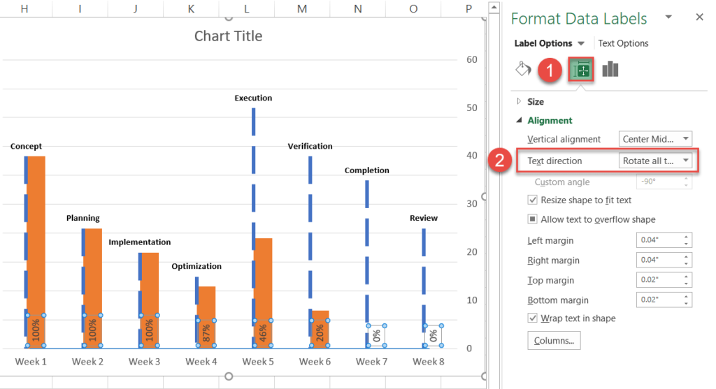
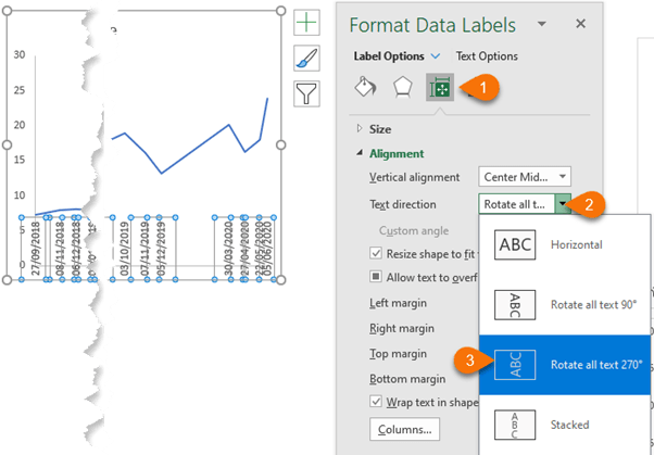
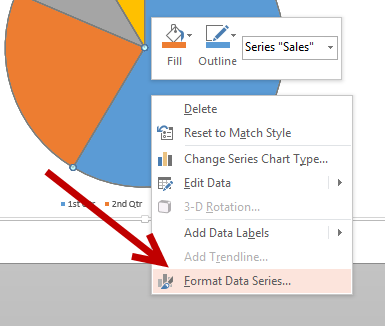
Rotate data labels excel chart. Change the format of data labels in a chart To format data labels, select your chart, and then in the Chart Design tab, click Add Chart Element > Data Labels > More Data Label Options. Click Label Options and under Label Contains, pick the options you want. To make data labels easier to read, you can move them inside the data points or even outside of the chart. Chart data-label rotation [SOLVED] - Excel Help Forum Chart data-label rotation. When working with a chart and wishing to rotate data labels, to do so manually I right click on a label, say "8:00", select "Format Labels", go down to "Alignment", select "Text Direction" drop-down, then from that select "Rotate all Text 90°" and I have what I want. Rotate chart data label Hi jujubeee, >> Rotate chart data label << Yes, we can set the custom angel for the data labe with DataLabel.Orientation Property. Here is an example that set the datalabel with custom angel (-40°) for your reference: ActiveChart.FullSeriesCollection(1).DataLabels.Select Selection.Orientation = 40 Custom Excel Chart Label Positions - YouTube Customize Excel Chart Label Positions with a ghost/dummy series in your chart. Download the Excel file and see step by step written instructions here: https:...
DataLabel.Orientation property (Excel) | Microsoft Docs In this article. Returns or sets a Variant value that represents the text orientation.. Syntax. expression.Orientation. expression A variable that represents a DataLabel object.. Remarks. The value of this property can be set to an integer value from -90 to 90 degrees or to one of the XlOrientation constants.. Support and feedback Is there a way to Slant data labels (rotate them) in a line graph? (Not ... Then, according to the "Re-positioning chart elements in Google Sheets" video example, I should be able to drag the single data label to a slightly different position near the corresponding data... Excel charts: add title, customize chart axis, legend and data labels ... Click anywhere within your Excel chart, then click the Chart Elements button and check the Axis Titles box. If you want to display the title only for one axis, either horizontal or vertical, click the arrow next to Axis Titles and clear one of the boxes: Click the axis title box on the chart, and type the text. How do i rotate the data labels in a histogram chart? I want the data labels in the histogram below to be vertical so that they become readable. However, the relevant options are "grayed out" as shown below. 884fabda-5de1-49a3-81e8-b1097fb7706d. 2273f8fb-3a59-4388-9f60-8510841bb339. Jakob Lunde.
Fantastic Rotate Data Labels Excel Line Graph Javascript Rotate data labels excel. The using the mouse looked at the Chart Option - Data Labels and found that Date Labels only have the following properties. The following is the chart. The icons to the left of the options show which way the text will rotate. Is it possible to do. Customize Excel Chart Label Positions with a ghostdummy series in your ... How to rotate charts in Excel - Basic Excel Tutorial Navigate to the " chart ribbon tools " and click it. 3. Proceed by selecting the " Format tab. ". 4. Select the drop-down menu on the top left corner and choose the vertical value axis. 5. The vertical axis is otherwise the value axis. Your next step is to identify the vertical axis of the chart that you want to rotate. › documents › excelHow to group (two-level) axis labels in a chart in Excel? The Pivot Chart tool is so powerful that it can help you to create a chart with one kind of labels grouped by another kind of labels in a two-lever axis easily in Excel. You can do as follows: 1. Create a Pivot Chart with selecting the source data, and: (1) In Excel 2007 and 2010, clicking the PivotTable > PivotChart in the Tables group on the ... Add / Move Data Labels in Charts - Excel & Google Sheets We'll start with the same dataset that we went over in Excel to review how to add and move data labels to charts. Add and Move Data Labels in Google Sheets. Double Click Chart; Select Customize under Chart Editor; Select Series . 4. Check Data Labels. 5. Select which Position to move the data labels in comparison to the bars. Final Graph with Google Sheets. After moving the dataset to the center, you can see the final graph has the data labels where we want.
E-xcel Tuts: Add Data Labels to Excel Charts
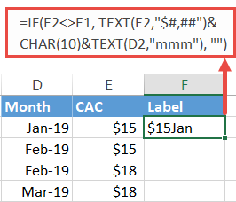
› 509290 › how-to-use-cell-valuesHow to Use Cell Values for Excel Chart Labels Mar 12, 2020 · Select the chart, choose the “Chart Elements” option, click the “Data Labels” arrow, and then “More Options.” Uncheck the “Value” box and check the “Value From Cells” box. Select cells C2:C6 to use for the data label range and then click the “OK” button.
![Custom Data Labels with Colors and Symbols in Excel Charts - [How To] - PakAccountants.com](https://pakaccountants.com/wp-content/uploads/2014/09/data-label-chart-6.gif)
Custom Data Labels with Colors and Symbols in Excel Charts - [How To] - PakAccountants.com
How to Add Total Data Labels to the Excel Stacked Bar Chart Step 4: Right click your new line chart and select "Add Data Labels" Step 5: Right click your new data labels and format them so that their label position is "Above"; also make the labels bold and increase the font size. Step 6: Right click the line, select "Format Data Series"; in the Line Color menu, select "No line"
How to Create a Timeline Chart in Excel - Automate Excel
How to I rotate data labels on a column chart so that they are ... To change the text direction, first of all, please double click on the data label and make sure the data are selected (with a box surrounded like following image). Then on your right panel, the Format Data Labels panel should be opened. Go to Text Options > Text Box > Text direction > Rotate.
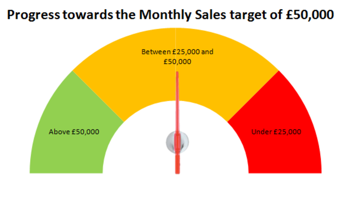
Creating a Speedometer, Dial or Gauge chart in Excel 2007 and Excel 2010 - HubPages
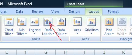
Add or remove data labels in a chart - support.microsoft.com Click the data series or chart. To label one data point, after clicking the series, click that data point. In the upper right corner, next to the chart, click Add Chart Element > Data Labels. To change the location, click the arrow, and choose an option. If you want to show your data label inside a text bubble shape, click Data Callout.
Adding data labels to see the value of the bars in an Excel chart
excel - Orientation of DataLabels - Stack Overflow cht.FullSeriesCollection(1).Select cht.FullSeriesCollection(1).ApplyDataLabels cht.FullSeriesCollection(1).DataLabels.Select Selection.Orientation = xlUpward Selection.Format.TextFrame2.Orientation = msoTextOrientationUpward 'In my case this will put the labels in the middle of the bars Selection.Position = xlLabelPositionCenter ' From here it is just more formatting With Selection.Format.TextFrame2.TextRange.Font.Fill .Visible = msoTrue .ForeColor.ObjectThemeColor = msoThemeColorBackground1 ...
How To Rotate Text In Excel Chart - Best Picture Of Chart Anyimage.Org
How to rotate axis labels in chart in Excel? Excel Functions; Excel Formulas; Excel Charts; Outlook Tutorials; Support. Online Tutorials Office Tab; Kutools for Excel; Kutools for Word; Kutools for Outlook; News and Updates Office Tab; Kutools for Excel; Kutools for Word; Kutools for Outlook; Search.
pgfplots - How to plot my data smoothly like excel does? - TeX - LaTeX Stack Exchange
› 07 › 09Rotate charts in Excel - spin bar, column, pie and line ... Therefore, the labels will be readable when the chart is rotated. Select the range of cells that contain your chart. Click on the Camera icon on the Quick Access toolbar . Click on any cell within your table to create a camera object. Now grab the Rotate control at the top. Rotate your chart in Excel to the needed angle and drop the control. Note.
Label Specific Excel Chart Axis Dates • My Online Training Hub
› 2015/11/12 › make-pie-chart-excelHow to make a pie chart in Excel - Ablebits Nov 12, 2015 · Showing data categories on the labels; Excel pie chart percentage and value; Adding data labels to Excel pie charts. In this pie chart example, we are going to add labels to all data points. To do this, click the Chart Elements button in the upper-right corner of your pie graph, and select the Data Labels option. Additionally, you may want to ...
PowerPoint: Rotate Pie Chart
Adjusting the Angle of Axis Labels (Microsoft Excel) If you are using Excel 2007 or Excel 2010, follow these steps: Right-click the axis labels whose angle you want to adjust. (You can only adjust the angle of all of the labels along an axis, not individual labels.) Excel displays a Context menu. Click the Format Axis option. Excel displays the Format Axis dialog box. (See Figure 1.) Figure 1.

Excel 2013 Tutorial for Beginners #65: Modifying Chart Axis, Labels, Gridlines, Etc. - YouTube
Rotate a Chart in Excel & Google Sheets - Automate Excel Rotate a Chart in Excel We'll start with the below bar graph that shows the Items sold by Year. Right click on X Axis Select Format Axis Change Angle of Label Click on the Size and Properties Tab Type in your Custom Angle. In this case, we'll say 30° And you'll see the chart with rotated axis: AutoMacro - VBA Code Generator Learn More

Data Labels | FusionCharts
How to Rotate Pie Chart in Excel? - WallStreetMojo To rotate the pie chart, click on the chart area. Right-click on the pie chart and select the "format data series" option. Change the angle of the first scale to 90 degrees to display the chart properly. Now the pie chart is looking good, representing clearly the small slices. Example #2 - 3D Rotate Pie Chart
Combine pie and xy scatter charts - Advanced Excel Charting Example | Chandoo.org - Learn ...
› charts › add-data-pointAdd Data Points to Existing Chart – Excel & Google Sheets Similar to Excel, create a line graph based on the first two columns (Months & Items Sold) Right click on graph; Select Data Range . 3. Select Add Series. 4. Click box for Select a Data Range. 5. Highlight new column and click OK. Final Graph with Single Data Point

How to avoid data label in excel line chart overlap with other line/label?

How to Create a Timeline Chart in Excel - Automate Excel
How to Create a Step Chart in Excel - Automate Excel
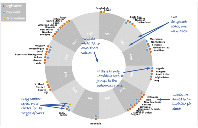
Combine pie and xy scatter charts - Advanced Excel Charting Example

Excel Chart Vertical Text Labels - YouTube
Post a Comment for "42 rotate data labels excel chart"