40 how to format data labels in excel charts

Walkthrough: Using Automation to Create a Graph in Microsoft Excel ... In the Project/Library list in the list box in the upper-left corner of the Object Browser, select Excel. In the Classes list, select XlWBATemplate. In the Members of 'XlWBATemplate' list, select xlWBATWorkSheet. You can see the value in the information pane at the bottom of the Object Browser. In the following example, the value is -4167.. How to make a 3 Axis Graph using Excel? - GeeksforGeeks A Format Data Series dialogue box appears. In the series Option, select the blue line as the Secondary Axis . Step 6: Now, you need to remove the Chart Title of graph1. Double click on the chart title of graph1. Format Chart Title dialogue box appears. Go to Text options. In the Text Fill, select No Fill.

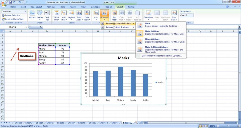
how to edit a legend in Excel — storytelling with data How to do it in Excel: Click on your graph, and then in your Excel ribbon, select the "Format" tab next to the "Chart Design" tab. Towards the left hand side of your ribbon, click on the icon of a text box. That will place a blank text box in your Chart Area, which you can move, edit, and format just like a regular text box.

How to format data labels in excel charts

How to make Excel graphs look professional & cool (10 charting tips) Go to Format in the Chart Tools context sensitive option In the Shape Styles group, click on the drop-down arrow for Shape Effects, choose Shadow, and then Perspective Diagonal Upper Right With your chart still selected, go to the Animations tab and do the following: In the Advanced Animation group, click to Add an Animation How To Calculate A CAGR In Excel (Correctly) While Excel doesn't have a function specifically called CAGR () in Excel, it does have a function we can utilize to calculate the CAGR metric. We can utilize the Excel Function RRI () to perform our calculation very easily. The RRI function (which stands for R ate of R eturn on I nvestment) utilizes the same 3 pieces of data used in the CAGR ... PBCharts Inflation Analysis - Peltier Tech Import Data into PBCharts: Click this button, then browse to a data file (CSV, TXT, or Excel) and PBCharts will import data from the selected file into a new PBCharts file. Analyze Selected Data in PBCharts: Select your data range, or select one cell in the data range, and click this button, and PBCharts will populate a new PBCharts file with the selected data, or if a single cell is selected ...

How to format data labels in excel charts. 14 Best Types of Charts and Graphs for Data Visualization - HubSpot Different Types of Graphs and Charts for Presenting Data. To better understand each chart and graph type and how you can use them, here's an overview of graph and chart types. 1. Bar Graph. A bar graph should be used to avoid clutter when one data label is long or if you have more than 10 items to compare. Best Use Cases for These Types of Graphs: A Beginner's Guide on How to Plot a Graph in Excel To format the headings, select the text in the title box. And then on the Home tab. Select the formatting style that you want. You can position the chart title above, below or any side of the graph. STEP 7: Adjust your data layout and colours Select the layout which you like the best as it gives your axes titles as well as your chart title. how to create a line chart in Excel — storytelling with data To begin, highlight the data table, including the column headers. To do this, click cell B7 and drag your cursor to C18. Next, navigate to the Insert ribbon and select the line chart icon. (Note that you can also use the Insert menu at the very top, then choose Chart -> Line to achieve a similar result.) Pivot Table data range in Excel - Microsoft Community After the data is loaded to Excel, in form of Excel Tables on a worksheet, the data can be manipulated in the table, or fed into a PivoTable and then to a PivotChart. PowerQuery allows you to use a "Click and Drag" user interface from the Ribbon and right click context menus to generate the required code in the background. .

A Step-by-Step Guide on How to Make a Graph in Excel Click on the chart TOOLS tab on the ribbon to add additional design and formatting capabilities and then click the options you desire under the DESIGN and FORMAT tabs. Creating a graph in Excel is easy. This step-by-step tutorial will show you how to make a graph in Excel. The demo helps you create: Bar Graph Pie Chart Scatter Plot 50 Excel Shortcuts That You Should Know in 2022 - Simplilearn Ctrl + Shift + Up Arrow. 25. To select all the cells below the selected cell. Ctrl + Shift + Down Arrow. In addition to the above-mentioned cell formatting shortcuts, let's look at a few more additional and advanced cell formatting Excel shortcuts, that might come handy. We will learn how to add a comment to a cell. Two level axis in Excel chart not showing • AuditExcel.co.za You can easily do this by: Right clicking on the horizontal access and choosing Format Axis Choose the Axis options (little column chart symbol) Click on the Labels dropdown Change the 'Specify Interval Unit' to 1 If you want you can make it look neater by ticking the Multi Level Category Labels How to Format Excel Pivot Table - Contextures Excel Tips In the Format Cells dialog box, select the Font, Border, and Fill settings you want for the selected element. Click OK, to return to the New PivotTable Quick Style dialog box, where the formatted element is listed with a bold font. In the screen shot below, you can see the revised color in the Preview section, at the right side of the dialog box..

Unlink Chart Data - Peltier Tech It's easy to link many of a chart's text elements to a worksheet range. Select the text element, click in the formula bar, type = and click on the cell or range containing the text you want displayed. The result is a link formula like =Sheet1!$A$1, and the text element updates dynamically to display whatever is in the reference. How to add secondary axis in Excel (2 easy ways) - ExcelDemy Go to Design tab (shows only when the chart is selected) => Type window => and click on the Change Chart Type command 5) Change Chart Type dialog box appears. This dialog box is actually our old Insert Chart dialog box. The Combo option is already selected. I just change the Chart Type from Clustered Column to Line with Markers. SPSS Tutorials: Frequency Tables - Kent State University SAS Syntax (*.sas) Syntax to read the CSV-format sample data and set variable labels and formats/value labels. Create a Frequency Table in SPSS In SPSS, the Frequencies procedure can produce summary measures for categorical variables in the form of frequency tables, bar charts, or pie charts. Conditional Formatting Shapes - Excel Dashboard School Let's go back to Sheet1. Highlight the object, and in the Formula Bar field, type in the following: =setup!$H$2 This will set the current value to 45. Then, based on the table, the shape will change its color to yellow because this value is between the upper and the lower value range.

Format Multiple Charts – Power BI & Excel are better together

linkedin-skill-assessments-quizzes/microsoft-excel-quiz.md at ... - GitHub Right-click column C, select Format Cells, and then select Best-Fit. Right-click column C and select Best-Fit. Double-click column C. Double-click the vertical boundary between columns C and D. Q2. Which two functions check for the presence of numerical or nonnumerical characters in cells? ISNUMBER and ISTEXT ISNUMBER and ISALPHA

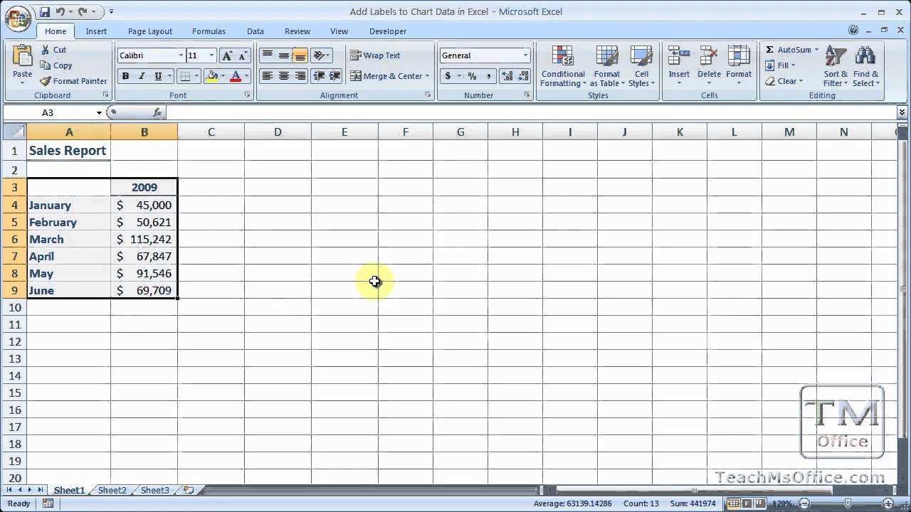
Add Labels to Chart Data in Excel - YouTube

Create Excel Waterfall Chart Template - Download Free Template Right-click on the scatter plot and select Add Data Labels. Right-click on the data labels and go to Format Data Labels. Under Label Options, check the box for Value from Cells and select cells D5 to D11 for the data label range. Uncheck other boxes for Label Options. Select Above for Label Positions.

Excel Dashboard Templates How-to Use Data Labels from a Range in an Excel Chart - Excel ...

Format Data | Reporting | DevExpress Documentation Format Data. This document describes how to apply standard .NET formats to data values in a report. After you bound your report to data and specified a bound data field in a report control's Expression property, you can format data values in a report. Invoke the control's smart tag and click the Format String property's ellipsis button ...

34 Label Chart In Excel - Labels Database 2020

Solved: Does Alteryx has Export-Excel Chart Function like ... - Alteryx ... Points 1-3 are dependent on how you configure the output data tool and points 4-5 need tools included in the reporting tool palette. However, your charts will not read data from the Raw Data tab but they will be static, so if someone opens that Excel and adds more data to the Raw Data tab, the charts won't update

How to Add Data Labels in Excel - Excelchat | Excelchat

Speedometer Chart in Excel | Microsoft Excel Tips | Excel Tutorial ... The default format of the chart Select the graph and on the Design tab, choose the Chart Styles group of the style that suits me. Formatting corrected by style With the chart still selected on the Layout tab, in the Labels group, click a legend and choose None. I note the green half circle by double clicking the left button.

Do My Excel Blog: How to design a multiple clustered bar chart series in Excel

Google Charts Hide Axis Labels - fpb.politecnico.lucca.it Double-click the line you want to graph on a secondary axis Include Charts 4 PHP Framework file & Initialize Object; Set the chart type and other options; Rendering Click the Tick Marks tab, select None for both Major tick marks and Minor tick marks, and then click OK Polar Legend . Show or hide the chart legend Show or hide the chart legend.

Custom Data Labels with Colors and Symbols in Excel Charts - [How To] - PakAccountants.com

How to Use Excel Pivot Table Label Filters Right-click on an item in the Row Labels or Column Labels In the pop-up menu, click Filter, then click Hide Selected Items. The item is immediately hidden in the pivot table. Quickly Hide All But a Few Items You can use a similar technique to hide most of the items in the Row Labels or Column Labels.

Do My Excel Blog: How to design a multiple clustered bar chart series in Excel

Types of Graphs - Top 10 Graphs for Your Data You Must Use Add data labels #8 Gauge Chart. The gauge chart is perfect for graphing a single data point and showing where that result fits on a scale from "bad" to "good." Gauges are an advanced type of graph, as Excel doesn't have a standard template for making them. To build one you have to combine a pie and a doughnut.

Basic Excel Chart Formatting - MS Excel Charting Tutorial Part 4 | Vertical Horizons

Create Radial Bar Chart in Excel - Step by step Tutorial First, create a helper column for the data labels on column E. Then enter the formula =B12&" ("&C12&")" on cell E12. You can use the CONCATENATE function also. Finally, fill down the formula for "E12:E16". Go to the Ribbon, and click on the Insert tab. Insert a Text box. Now we'll create a linked cell to the Text box.

34 Data Label In Excel Chart - Labels For Your Ideas

PBCharts Inflation Analysis - Peltier Tech Import Data into PBCharts: Click this button, then browse to a data file (CSV, TXT, or Excel) and PBCharts will import data from the selected file into a new PBCharts file. Analyze Selected Data in PBCharts: Select your data range, or select one cell in the data range, and click this button, and PBCharts will populate a new PBCharts file with the selected data, or if a single cell is selected ...

Format Number Options for Chart Data Labels in Excel 2011 for Mac

How To Calculate A CAGR In Excel (Correctly) While Excel doesn't have a function specifically called CAGR () in Excel, it does have a function we can utilize to calculate the CAGR metric. We can utilize the Excel Function RRI () to perform our calculation very easily. The RRI function (which stands for R ate of R eturn on I nvestment) utilizes the same 3 pieces of data used in the CAGR ...