41 excel chart hide zero labels

How to Hide Zero Values in Excel Pivot Table (3 Easy Methods) So, if your goal is to hide zero values but don't want to hide cells, you can certainly use this method. Just follow these simple steps below: 📌 Steps ① First, select the entire table. ② Then, press Ctrl+1 on your keyboard to open the Format Cells dialog box. Next, select Custom. ③ After that, clear the General from the Type field. Make Excel charts primary and secondary axis the same scale To hide the series all you need to do is tell each series to have no fill, border and line (depending on how they are showing). These series may be hard to see so the easiest way to customise them is to click on the Chart, click on the Format tab, and find the series called Primary Scale.

Excel hide chart axis labels Archives - Data Cornering Tag: Excel hide chart axis labels. DataViz Excel. How to add text labels on Excel scatter chart axis. by Janis Sturis July 11, 2022 Comments 0. Categories.

Excel chart hide zero labels

How to get Excel Chart Columns with no gaps - AuditExcel.co.za In order to do this you can right click on any one of the data series and choose Format Data Series. You will notice that one of the options is Gap Width and the default is 150%. You can play with this gap width but the extreme would be to remove the gap completely (make it 0%) as shown below. Removing gaps between bars in an Excel chart - TheSmartMethod.com 1. Open the Format Data Series task pane Right-click on one of the bars in your chart and click Format Data Series from the shortcut menu. The Format Data Series task pane appears on the right-hand side of the screen, offering many different options. Excel / Auto Hide Rows - Microsoft Tech Community Re: Excel / Auto Hide Rows. @Taylor_Watson. Depends in part on what you mean by "Hides" and on the bigger picture into which this request fits. Assuming that it's the value in the cell in column A, which, if it's 3, is cause for none of the other cells to be displayed, you could always add an IF condition to each of the other cells in the row ...

Excel chart hide zero labels. Unable to show gaps for empty cells when plotting chart Report Inappropriate Content. Nov 26 2017 09:01 PM. Re: Unable to show gaps for empty cells when plotting chart. This depends on the type of chart you have. In stacked line chart or a 100% stacked line chart you only have zero option. 1 Like. How to Refresh Chart in Excel (2 Effective Ways) - ExcelDemy Let's follow the instructions below to refresh a chart! Step 1: First of all, select the data range. From our dataset, we will select B4 to D10 for the convenience of our work. Hence, from your Insert tab, go to, Insert → Tables → Table As a result, a Create Table dialog box will appear in front of you. From the Create Table dialog box, press OK. Show/Hide Field Headers in Excel Pivot Tables - MyExcelOnline STEP 1: Go to PivotTable Analyze > Show > Field Headers Click on it to hide the field headers: And they are now hidden! You can click on the same button to show them again. The headers will be visible again! HELPFUL RESOURCE: Make sure to download our FREE PDF on the 333 Excel keyboard Shortcuts here: Excel Waterfall Chart: How to Create One That Doesn't Suck To create a waterfall chart in Excel 2013 and earlier, you had to define additional data series (with complicated formulas) in the data table and then make them invisible in the chart. And we're not talking about 1 invisible series. If the waterfall chart dipped below zero at one point, you needed at least seven additional series!

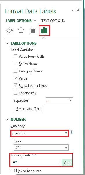
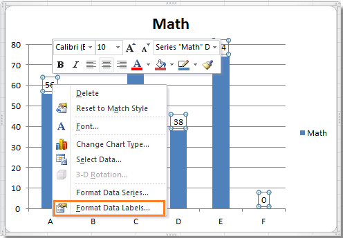
› documents › excelHow to hide zero data labels in chart in Excel? - ExtendOffice In the Format Data Labelsdialog, Click Numberin left pane, then selectCustom from the Categorylist box, and type #""into the Format Codetext box, and click Addbutton to add it to Typelist box. See screenshot: 3. Click Closebutton to close the dialog. Then you can see all zero data labels are hidden. How to Change the X-Axis in Excel - Alphr Open the Excel file with the chart you want to adjust. Right-click the X-axis in the chart you want to change. That will allow you to edit the X-axis specifically. Then, click on Select Data. Next ... Custom Excel number format - Ablebits.com To hide a certain value type(s), skip the corresponding code section, and only type the ending semicolon. For example, to hide zeros and negative values, use the following format code: General; ; ; General. As the result, zeros and negative value will appear only in the formula bar, but will not be visible in cells. Bubble Chart in Excel chart or Excel Pivot Chart Select the X-axis, change the minimum value to 0, and change the axis label position to No Labels. Repeat for the Y-axis, and you'll have chart 4. Select the X-axis labels, press Ctrl+1 to format them.

How to Create and Customize a Waterfall Chart in Microsoft Excel To fix this, double-click the chart to display the Format sidebar. Select the bar for the total by clicking it twice. Click the Series Options tab in the sidebar and expand Series Options if necessary. Check the box for "Set as Total." Then, do the same for the other total. excel - How to not display labels in pie chart that are 0% - Stack Overflow Generate a new column with the following formula: =IF (B2=0,"",A2) Then right click on the labels and choose "Format Data Labels". Check "Value From Cells", choosing the column with the formula and percentage of the Label Options. Under Label Options -> Number -> Category, choose "Custom". Under Format Code, enter the following: How to avoid data label in excel line chart overlap ... - Stack Overflow However, it seems like the data labels will overlap with either the green dot/red dot/line. If I adjust the position of the data labels, it will only work for this 2 series of values. Sometime the values will change and cause the purple line to be above the black line, and then the data labels overlap with something else again. Change Primary Axis in Excel - Excel Tutorials To hide the y-axis we follow the steps below: Click anywhere in the chart to display the Chart Tools tab together with the Design and Format tabs: Click Chart Tools >> Design >> Add Chart Element >> Axes >> Primary Vertical on the Excel Ribbon: The vertical axis is hidden:

Excel Chart Axis Label Tricks • My Online Training Hub

› article › how-to-suppress-0How to suppress 0 values in an Excel chart - TechRepublic Jul 20, 2018 · Here’s how: Click the File tab and choose Options. In Excel 2007, click the Office button and then click Excel options. In Excel... Choose Advanced in the left pane. In the Display options for this worksheet section, choose the appropriate sheet from the drop-down menu. Uncheck the Show a zero in ...

32 How To Label Graphs In Excel - Labels Database 2020

Formatting Long Labels in Excel - PolicyViz Open PowerPoint and Paste the graph. Don't worry about the slide size or anything, just paste it in. Select the axis you want to format and select the Format option in the Paragraph menu. In the ensuing menu, select the Right option in the Alignment drop-down menu. Now, ideally, we'd be able to align the text to the left and everything ...

Area Chart - Invert if Negative - Peltier Tech Blog

How to Change the Y Axis in Excel - Alphr Go to "Design," then go to "Add Chart Element" and "Axes." You'll have two options: "Primary Horizontal" will hide/unhide the horizontal axis, and if you choose "Primary Vertical," it will...

Display Zero Values In Pivot Chart - Best Picture Of Chart Anyimage.Org

How to: Show or Hide the Chart Legend - DevExpress However, to save space in the chart, you can turn this option off by setting the Legend.Overlay property to true. To remove the legend completely, set the Legend.Visible property to false. Worksheet worksheet = workbook.Worksheets ["chartTask3"]; workbook.Worksheets.ActiveWorksheet = worksheet; // Create a chart and specify its location.

How to add total labels to stacked column chart in Excel?

› documents › excelHow to hide zero data labels in chart in Excel? - ExtendOffice Tip: If you want to show the zero data labels, please go back to Format Data Labels dialog, and click Number > Custom, and select #,##0;-#,##0 in the Type list box. Note: In Excel 2013, you can right click the any data label and select Format Data Labels to open the Format Data Labels pane; then click Number to expand its option; next click the ...

How to hide zero data labels in chart in Excel?

How to Apply a Filter to a Chart in Microsoft Excel Go to the Home tab, click the Sort & Filter drop-down arrow in the ribbon, and choose "Filter.". Click the arrow at the top of the column for the chart data you want to filter. Use the Filter section of the pop-up box to filter by color, condition, or value. When you finish, click "Apply Filter" or check the box for Auto Apply to see ...

How to hide zero data labels in chart in Excel?

How to format axis labels individually in Excel - SpreadsheetWeb Excluding Zero [Green]; [Red];0 Showing individual items By using condition-type syntax, you can display selective items. Displaying a single value The following code formats axis items equal to 60 to color Cyan. [Cyan] [=60]; There are two important point with this code: There must be an item which is equals to 60 on the axis.

32 How To Label A Graph In Excel - Labels Database 2020

Chart.Axes method (Excel) | Microsoft Docs This example adds an axis label to the category axis on Chart1. VB. With Charts ("Chart1").Axes (xlCategory) .HasTitle = True .AxisTitle.Text = "July Sales" End With. This example turns off major gridlines for the category axis on Chart1. VB.

30 How To Add Label To Excel Chart - Labels Database 2020

TickLabels object (Excel) | Microsoft Docs Example. Use the TickLabels property of the Axis object to return the TickLabels object. The following example sets the number format for the tick-mark labels on the value axis in embedded chart one on Sheet1. Worksheets ("sheet1").ChartObjects (1).Chart _ .Axes (xlValue).TickLabels.NumberFormat = "0.00".

Excel Chart With Irregular Horizontal Bands - Peltier Tech Blog

Modifying Axis Scale Labels (Microsoft Excel) Follow these steps: Create your chart as you normally would. Double-click the axis you want to scale. You should see the Format Axis dialog box. (If double-clicking doesn't work, right-click the axis and choose Format Axis from the resulting Context menu.) Make sure the Number tab is displayed. (See Figure 1.) Figure 1.

Fixing Your Excel Chart When the Multi-Level Category Label Option is Missing. - Excel Dashboard ...

How to Use Excel Pivot Table Label Filters Instead of searching through a long list of items in a drop down list, you can use a quick command to hide the selected items. Right-click on an item in the Row Labels or Column Labels In the pop-up menu, click Filter, then click Hide Selected Items. The item is immediately hidden in the pivot table. Quickly Hide All But a Few Items

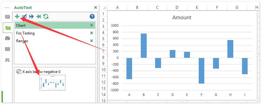
How to move chart X axis below negative values/zero/bottom in Excel?

I do not want to show data in chart that is "0" (zero) To access these options, select the chart and click: Chart Tools > Design > Select Data > Hidden and Empty Cells You can use these settings to control whether empty cells are shown as gaps or zeros on charts. With Line charts you can choose whether the line should connect to the next data point if a hidden or empty cell is found.

How to Edit Legend in Excel (Visual Tutorial) | Blog | Whatagraph

Excel / Auto Hide Rows - Microsoft Tech Community Re: Excel / Auto Hide Rows. @Taylor_Watson. Depends in part on what you mean by "Hides" and on the bigger picture into which this request fits. Assuming that it's the value in the cell in column A, which, if it's 3, is cause for none of the other cells to be displayed, you could always add an IF condition to each of the other cells in the row ...

I only want to see actual x values to show on horizontal axis of Excel Chart (with scale ...

Removing gaps between bars in an Excel chart - TheSmartMethod.com 1. Open the Format Data Series task pane Right-click on one of the bars in your chart and click Format Data Series from the shortcut menu. The Format Data Series task pane appears on the right-hand side of the screen, offering many different options.