44 add data labels to excel chart
How to add Data label in Stacked column chart of Pivot charts Hello friends, I'm tring to make a Pivot chart with stacked column graph. In where, i couldn't add data label for cumulative sum of value in Data label. Where i could only add data label to individual stacks in column graph. It found possible with normal stacked column chart without pivot chart. DataLabels object (Excel) | Microsoft Docs The following example sets the number format for data labels on series one on chart sheet one. With Charts(1).SeriesCollection(1) .HasDataLabels = True .DataLabels.NumberFormat = "##.##" End With Use DataLabels (index), where index is the data-label index number, to return a single DataLabel object. The following example sets the number format ...
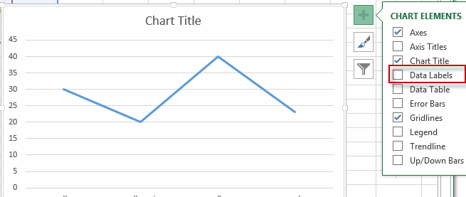
How to Add Leader Lines in Excel? - GeeksforGeeks Step 2: Go to Insert Tab and select Recommended Charts. A dialogue box name Insert Chart appears. Step 3: Click on All Charts and select Line. Click Ok. Step 4: A line chart is embedded in the worksheet. Step 5: Go to Chart Design Tab and select Add Chart Element . Step 6: Hover on the Data Labels option. Click on More Data Label Options ….

Add data labels to excel chart
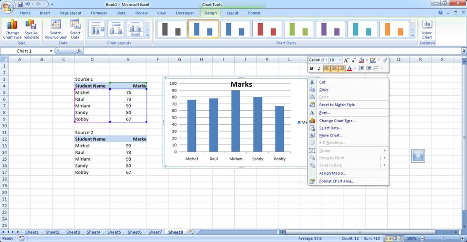
How to Make a Pie Chart in Excel & Add Rich Data Labels to The Chart! 8) With the one data point still selected, right-click this data point, and select Add Data Label>Add Data Callout as shown below. 9) Select only this data label and right-click and choose Insert Data Label Field as shown below. 10) Select [Cell] Choose Cell from the options. How to Add Total Values to Stacked Bar Chart in Excel Step 4: Add Total Values. Next, right click on the yellow line and click Add Data Labels. Next, double click on any of the labels. In the new panel that appears, check the button next to Above for the Label Position: Next, double click on the yellow line in the chart. In the new panel that appears, check the button next to No line: › documents › excelHow to add or move data labels in Excel chart? - ExtendOffice Add or move data labels in Excel chart. 1. Click the chart to show the Chart Elements button . 2. Then click the Chart Elements, and check Data Labels, then you can click the arrow to choose an option about the data labels in the sub menu. See ... 1. click on the chart to show the Layout tab in the ...
Add data labels to excel chart. How to Add a Vertical Line to Charts in Excel - Statology Step 1: Enter the Data. Suppose we would like to create a line chart using the following dataset in Excel: Step 2: Add Data for Vertical Line. Now suppose we would like to add a vertical line located at x = 6 on the plot. We can add in the following artificial (x, y) coordinates to the dataset: Step 3: Create Line Chart with Vertical Line How To Create Labels In Excel . look serenity 2022 How To Create Labels In Excel. There are a few different techniques we could use to create labels that look like this. Once you have the excel spreadsheet and. How To Create Labels In Excel. There are a few different techniques we could use to create labels that look like this. ... Add custom text here or remove it. Search for: Home; Cookie ... How To Add Data Labels In Excel ~ 2022 Right click the data series in the chart, and select add data labels > add data labels from the context menu to add data labels. Then click the chart elements, and check data labels, then you can click the arrow to choose an option about the data labels in the sub menu. Source: In excel 2013 or 2016. DataLabel object (Excel) | Microsoft Docs The following example turns on the data label for the second point in series one on the chart sheet named Chart1, and sets the data label text to Saturday. VB With Charts ("chart1") With .SeriesCollection (1).Points (2) .HasDataLabel = True .DataLabel.Text = "Saturday" End With End With
How to Edit Pie Chart in Excel (All Possible Modifications) How to Edit Pie Chart in Excel 1. Change Chart Color 2. Change Background Color 3. Change Font of Pie Chart 4. Change Chart Border 5. Resize Pie Chart 6. Change Chart Title Position 7. Change Data Labels Position 8. Show Percentage on Data Labels 9. Change Pie Chart's Legend Position 10. Edit Pie Chart Using Switch Row/Column Button 11. support.microsoft.com › en-us › officeAdd or remove data labels in a chart - support.microsoft.com Add data labels to a chart Click the data series or chart. To label one data point, after clicking the series, click that data point. In the upper right corner, next to the chart, click Add Chart Element > Data Labels. To change the location, click the arrow, and choose an option. If you want to ... How to make a quadrant chart using Excel - Basic Excel Tutorial Format data labels. Right-click on any label and select 'Format Data Labels.' Go to the 'Label Options' tab and check the 'Value from cells' option. Select all the names and click OK. Uncheck the 'Y Value' box and under 'Label Position,' select 'Above. 7. Add the Axis titles. Select the chart and go to the 'Design' tab. Choose 'Add Chart ... How to Add Labels to Scatterplot Points in Excel - Statology Step 3: Add Labels to Points Next, click anywhere on the chart until a green plus (+) sign appears in the top right corner. Then click Data Labels, then click More Options… In the Format Data Labels window that appears on the right of the screen, uncheck the box next to Y Value and check the box next to Value From Cells.
Point.DataLabel property (Excel) | Microsoft Docs In this article. Returns a DataLabel object that represents the data label associated with the point. Read-only. Syntax. expression.DataLabel. expression A variable that represents a Point object.. Example. This example turns on the data label for point seven in series three on Chart1, and then it sets the data label color to blue. How to add text labels on Excel scatter chart axis - Data Cornering Stepps to add text labels on Excel scatter chart axis 1. Firstly it is not straightforward. Excel scatter chart does not group data by text. Create a numerical representation for each category like this. By visualizing both numerical columns, it works as suspected. The scatter chart groups data points. 2. Secondly, create two additional columns. Excel: How to Create a Bubble Chart with Labels - Statology Step 3: Add Labels. To add labels to the bubble chart, click anywhere on the chart and then click the green plus "+" sign in the top right corner. Then click the arrow next to Data Labels and then click More Options in the dropdown menu: In the panel that appears on the right side of the screen, check the box next to Value From Cells within ... How to use cell values for excel chart labels - How to We want to chart the sales values and use the change values for data labels. Use Cell Values for Chart Data Labels. Select range A1:B6 and click Insert > Insert Column or Bar Chart > Clustered Column. The column chart will appear. We want to add data labels to show the change in value for each product compared to last month. Select the chart ...
How to Make Excel Charts More Intuitive by Adding Data Labels and ...
Add Vertical Lines To Excel Charts Like A Pro! [Guide] After you've re-jiggered your vertical line setup, you can then proceed to add a data label. Simply select your plotted dot and right-click on it. Then open the Add Data Labels menu and click Add Data Labels. You should then see a data label appear next to your vertical line.
How to label graphs in Excel | Think Outside The Slide
› documents › excelHow to add data labels from different column in an Excel chart? Batch add all data labels from different column in an Excel chart. 1. Right click the data series in the chart, and select Add Data Labels > Add Data Labels from the context menu to add data labels. 2. Right click the data series, and select Format Data Labels from the context menu. 3. In the Format ...
Adding data lables to see the value of the bars in an Excel chart
support.microsoft.com › en-us › officeEdit titles or data labels in a chart - support.microsoft.com Reestablish a link to data on the worksheet. On a chart, click the label that you want to link to a corresponding worksheet cell. On the worksheet, click in the formula bar, and then type an equal sign (=). Select the worksheet cell that contains the data or text that you want to display in your ...

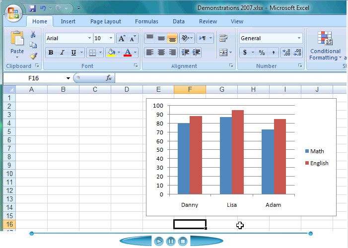
How to Create a Chart in Microsoft Excel - TechSupport
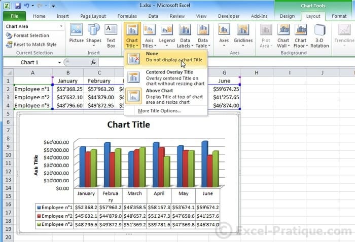
› how-to-add-data-labels-in-excelHow to Add Data Labels in Excel - Excelchat | Excelchat After inserting a chart in Excel 2010 and earlier versions we need to do the followings to add data labels to the chart; Click inside the chart area to display the Chart Tools. Figure 2. Chart Tools Click on Layout tab of the Chart Tools. In Labels group, click on Data Labels and select the position to add labels to the chart. Figure 3.
Add Data Labels in a Chart - Free Excel Tutorial
How to add a single vertical bar to a Microsoft Excel line chart You might add data labels or use pictures instead of a plain column in a column chart. One clever visual tool for highlighting a specific chart element or data point is to add a vertical bar. It...
Excel Course: Inserting Graphs
excel - Formatting Data Labels on a Chart - Stack Overflow sub charttest () activesheet.chartobjects ("chart 6").activate z = 1 with activechart if .charttype = xlline then i = .seriescollection (1).points.count activechart.fullseriescollection (1).datalabels.select for pts = 1 to i activechart.fullseriescollection (1).points (pts).hasdatalabel = true ' make sure all points are visible data …
Basic Excel Chart Formatting - MS Excel Charting Tutorial Part 4 ...
How to Create and Customize a Treemap Chart in Microsoft Excel Simply click that text box and enter a new name. Next, you can select a style, color scheme, or different layout for the treemap. Select the chart and go to the Chart Design tab that displays. Use the variety of tools in the ribbon to customize your treemap. For fill and line styles and colors, effects like shadow and 3-D, or exact size and ...
How to Create a Step Chart in Excel - Automate Excel
How to Create and Customize a Waterfall Chart in Microsoft Excel Select the chart and use the buttons on the right (Excel on Windows) to adjust Chart Elements like labels and the legend, or Chart Styles to pick a theme or color scheme. Select the chart and go to the Chart Design tab. Then, use the tools in the ribbon to select a different layout, change the colors, pick a new style, or adjust your data ...
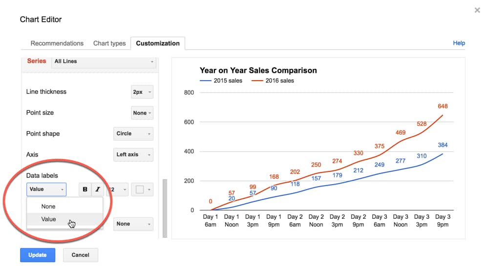
How can I annotate data points in Google Sheets charts? - Ben Collins
How to Apply a Filter to a Chart in Microsoft Excel Select the data for your chart, not the chart itself. Go to the Home tab, click the Sort & Filter drop-down arrow in the ribbon, and choose "Filter." Click the arrow at the top of the column for the chart data you want to filter. Use the Filter section of the pop-up box to filter by color, condition, or value.
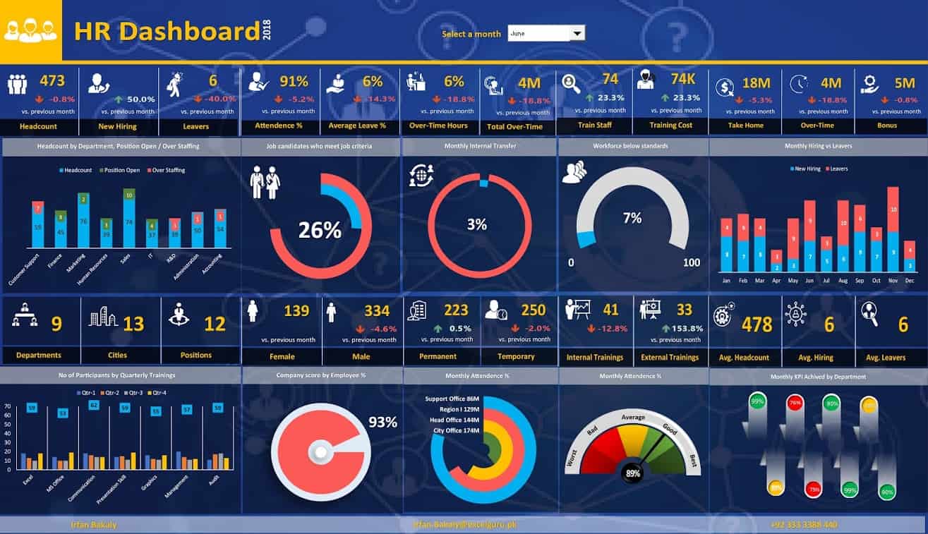
Excel Advanced Dashboard
How To Add Data Labels In Excel . Adopteesearch July To format data labels, select your chart, and then in the chart design tab, click add chart element > data labels > more data label options. Select Each Item Where You Want The Custom Label One At A Time. Excel provides several options for the placement and formatting of data labels. Press the ok button to close the change chart type dialog box.

excel - How do I update the data label of a chart? - Stack Overflow
Chart.ApplyDataLabels method (Excel) | Microsoft Docs ApplyDataLabels ( Type, LegendKey, AutoText, HasLeaderLines, ShowSeriesName, ShowCategoryName, ShowValue, ShowPercentage, ShowBubbleSize, Separator) expression A variable that represents a Chart object. Parameters Example This example applies category labels to series one on Chart1. VB Copy Charts ("Chart1").SeriesCollection (1).

Enable or Disable Excel Data Labels at the click of a button - How To ...
Line Chart in Excel | Microsoft Excel Tips | Excel Tutorial | Free ... Click on the data series, right-click and choose Select Data. In the dialog box that appears, edit the horizontal axis labels. Then choose the range axis labels. Simply select the year from the table data. Now the data series in the chart now looks as it should. Your line chart is ready. If necessary, Excel allows us to next modify the chart.

Excel Charts Archives - PakAccountants.com
How do I add labels to Gantt Chart? - Power BI You can create a measure like this one that has both values and then use that as your data label. DataLabel = MIN (Sheet1 [Leaving Date]) & " - " & MIN (Sheet1 [Returning Date]) Pat. Did I answer your question? Mark my post as a solution! Kudos are also appreciated!
Panel Bar Chart in Excel with 3 sets of data - XcelanZ
Series.DataLabels method (Excel) | Microsoft Docs This example sets the data labels for series one on Chart1 to show their key, assuming that their values are visible when the example runs. VB Copy With Charts ("Chart1").SeriesCollection (1) .HasDataLabels = True With .DataLabels .ShowLegendKey = True .Type = xlValue End With End With Support and feedback

How to Add Data Labels to an Excel 2010 Chart - dummies
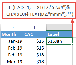
Custom Chart Data Labels In Excel With Formulas Follow the steps below to create the custom data labels. Select the chart label you want to change. In the formula-bar hit = (equals), select the cell reference containing your chart label's data. In this case, the first label is in cell E2. Finally, repeat for all your chart laebls.
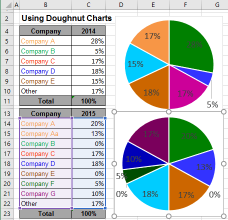
Using Pie Charts and Doughnut Charts in Excel
› documents › excelHow to add or move data labels in Excel chart? - ExtendOffice Add or move data labels in Excel chart. 1. Click the chart to show the Chart Elements button . 2. Then click the Chart Elements, and check Data Labels, then you can click the arrow to choose an option about the data labels in the sub menu. See ... 1. click on the chart to show the Layout tab in the ...
Post a Comment for "44 add data labels to excel chart"