44 how to add multiple data labels in excel

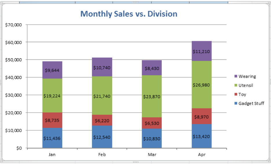
How can I add data labels from a third column to a scatterplot? Under Labels, click Data Labels, and then in the upper part of the list, click the data label type that you want. Under Labels, click Data Labels, and then in the lower part of the list, click where you want the data label to appear. Depending on the chart type, some options may not be available. Add / Move Data Labels in Charts - Excel & Google Sheets Check Data Labels . Change Position of Data Labels. Click on the arrow next to Data Labels to change the position of where the labels are in relation to the bar chart. Final Graph with Data Labels. After moving the data labels to the Center in this example, the graph is able to give more information about each of the X Axis Series.

how to add data labels into Excel graphs - storytelling with data You can download the corresponding Excel file to follow along with these steps: Right-click on a point and choose Add Data Label. You can choose any point to add a label—I'm strategically choosing the endpoint because that's where a label would best align with my design. Excel defaults to labeling the numeric value, as shown below.

How to add multiple data labels in excel

Add a DATA LABEL to ONE POINT on a chart in Excel Steps shown in the video above: Click on the chart line to add the data point to. All the data points will be highlighted. Click again on the single point that you want to add a data label to. Right-click and select ' Add data label ' This is the key step! Right-click again on the data point itself (not the label) and select ' Format data label '. Multiple data labels (in separate locations on chart) Re: Multiple data labels (in separate locations on chart) You can do it in a single chart. Create the chart so it has 2 columns of data. At first only the 1 column of data will be displayed. Move that series to the secondary axis. You can now apply different data labels to each series. Attached Files 819208.xlsx‎ (13.8 KB, 265 views) Download How to group (two-level) axis labels in a chart in Excel? - ExtendOffice (1) In Excel 2007 and 2010, clicking the PivotTable > PivotChart in the Tables group on the Insert Tab; (2) In Excel 2013, clicking the Pivot Chart > Pivot Chart in the Charts group on the Insert tab. 2. In the opening dialog box, check the Existing worksheet option, and then select a cell in current worksheet, and click the OK button. 3.

How to add multiple data labels in excel. Edit titles or data labels in a chart - support.microsoft.com To edit the contents of a title, click the chart or axis title that you want to change. To edit the contents of a data label, click two times on the data label that you want to change. The first click selects the data labels for the whole data series, and the second click selects the individual data label. Click again to place the title or data ... How to Add Multiple Cells in Excel (6 Methods) - ExcelDemy The SUM function is one of the most simple ways to add multiple cells in Excel easily. Type " =SUM ( " in Cell C10. Now we can manually input the data by using a comma for each. Or by clicking and dragging data cells that contain values we want to add. After hitting the Enter, we can easily find the required result. Add a label or text box to a worksheet - support.microsoft.com You can add labels to forms and ActiveX controls. Add a label (Form control) Click Developer, click Insert, and then click Label . Click the worksheet location where you want the upper-left corner of the label to appear. To specify the control properties, right-click the control, and then click Format Control. Add a label (ActiveX control) Multi Level Data Labels in Charts - Beat Excel! A better approach is to format modify your data make multiple levels of labels before generating your chart. This way your chart will look much more professional. You don't need to make anything else. After modifying your data, just select all data as you did before and insert your chart.

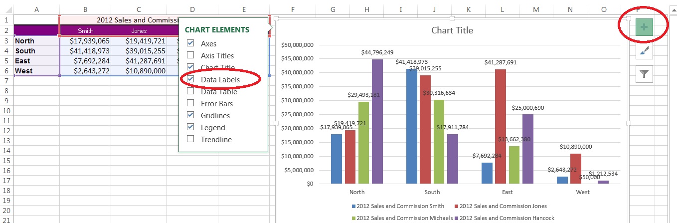
How to add or move data labels in Excel chart? - ExtendOffice In Excel 2013 or 2016. 1. Click the chart to show the Chart Elements button . 2. Then click the Chart Elements, and check Data Labels, then you can click the arrow to choose an option about the data labels in the sub menu. See screenshot: Format Data Labels in Excel- Instructions - TeachUcomp, Inc. To format data labels in Excel, choose the set of data labels to format. To do this, click the "Format" tab within the "Chart Tools" contextual tab in the Ribbon. Then select the data labels to format from the "Chart Elements" drop-down in the "Current Selection" button group. Then click the "Format Selection" button that ... Add data labels and callouts to charts in Excel 365 - EasyTweaks.com Step #1: After generating the chart in Excel, right-click anywhere within the chart and select Add labels . Note that you can also select the very handy option of Adding data Callouts. Step #2: When you select the "Add Labels" option, all the different portions of the chart will automatically take on the corresponding values in the table ... How to Add Data Labels in Excel - Excelchat | Excelchat In Excel 2013 and the later versions we need to do the followings; Click anywhere in the chart area to display the Chart Elements button Figure 5. Chart Elements Button Click the Chart Elements button > Select the Data Labels, then click the Arrow to choose the data labels position. Figure 6. How to Add Data Labels in Excel 2013 Figure 7.

Adding rich data labels to charts in Excel 2013 | Microsoft 365 Blog To add a data label in a shape, select the data point of interest, then right-click it to pull up the context menu. Click Add Data Label, then click Add Data Callout . The result is that your data label will appear in a graphical callout. In this case, the category Thr for the particular data label is automatically added to the callout too. How to Create a Graph with Multiple Lines in Excel Click Select Data button on the Design tab to open the Select Data Source dialog box. Select the series you want to edit, then click Edit to open the Edit Series dialog box. Type the new series label in the Series name: textbox, then click OK. Creating & Labeling Small Multiple Bar Charts in Excel Add data labels to your gap data bar Select format data labels Choose "value from cells" in the formatting panel Highlight the data from the real category adjacent to the gap data Uncheck "value" and "show leader lines" Change the label position to "inside base" Step 5: Add at title and category labels The final step is all about formatting. How to Add Data Labels to an Excel 2010 Chart - dummies On the Chart Tools Layout tab, click Data Labels→More Data Label Options. The Format Data Labels dialog box appears. You can use the options on the Label Options, Number, Fill, Border Color, Border Styles, Shadow, Glow and Soft Edges, 3-D Format, and Alignment tabs to customize the appearance and position of the data labels.

Enable or Disable Excel Data Labels at the click of a button - How To - PakAccountants.com

How to add data labels from different column in an Excel chart? Right click the data series in the chart, and select Add Data Labels > Add Data Labels from the context menu to add data labels. 2. Click any data label to select all data labels, and then click the specified data label to select it only in the chart. 3.

Enable or Disable Excel Data Labels at the click of a button - How To - PakAccountants.com

Add or remove data labels in a chart - support.microsoft.com Right-click the data series or data label to display more data for, and then click Format Data Labels. Click Label Options and under Label Contains, select the Values From Cells checkbox. When the Data Label Range dialog box appears, go back to the spreadsheet and select the range for which you want the cell values to display as data labels.

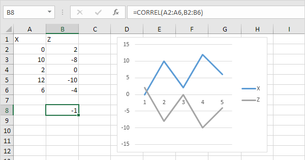
Correlation Analysis - Easy Excel Tutorial

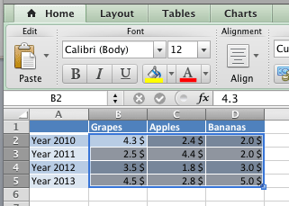
Plot Multiple Data Sets on the Same Chart in Excel Follow the below steps to implement the same: Step 1: Insert the data in the cells. After insertion, select the rows and columns by dragging the cursor. Step 2: Now click on Insert Tab from the top of the Excel window and then select Insert Line or Area Chart. From the pop-down menu select the first "2-D Line".

Format Number Options for Chart Data Labels in Excel 2011 for Mac

How to Add Axis Labels in Excel Charts - Step-by-Step (2022) - Spreadsheeto How to add axis titles 1. Left-click the Excel chart. 2. Click the plus button in the upper right corner of the chart. 3. Click Axis Titles to put a checkmark in the axis title checkbox. This will display axis titles. 4. Click the added axis title text box to write your axis label.

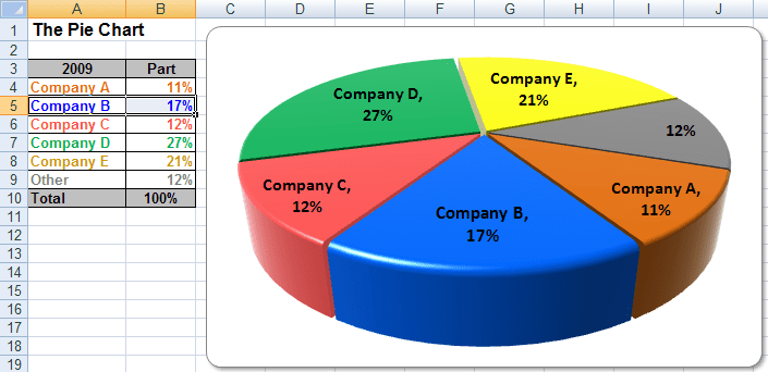
Excel 3-D Pie Charts

How to add multiple data label in Line Chart - Power BI you cannot add two data labels directly to your line chart on a single line, because the data labels are refering to that specific point, one option is to add it as a tooltip another option is to add a new line with the value you want and then make the line invisible and just show the data lable, be aware that depending on the information you …

How to Add Data Labels in Excel - Excelchat | Excelchat

How to Print Labels from Excel - Lifewire Select Mailings > Write & Insert Fields > Update Labels . Once you have the Excel spreadsheet and the Word document set up, you can merge the information and print your labels. Click Finish & Merge in the Finish group on the Mailings tab. Click Edit Individual Documents to preview how your printed labels will appear. Select All > OK .

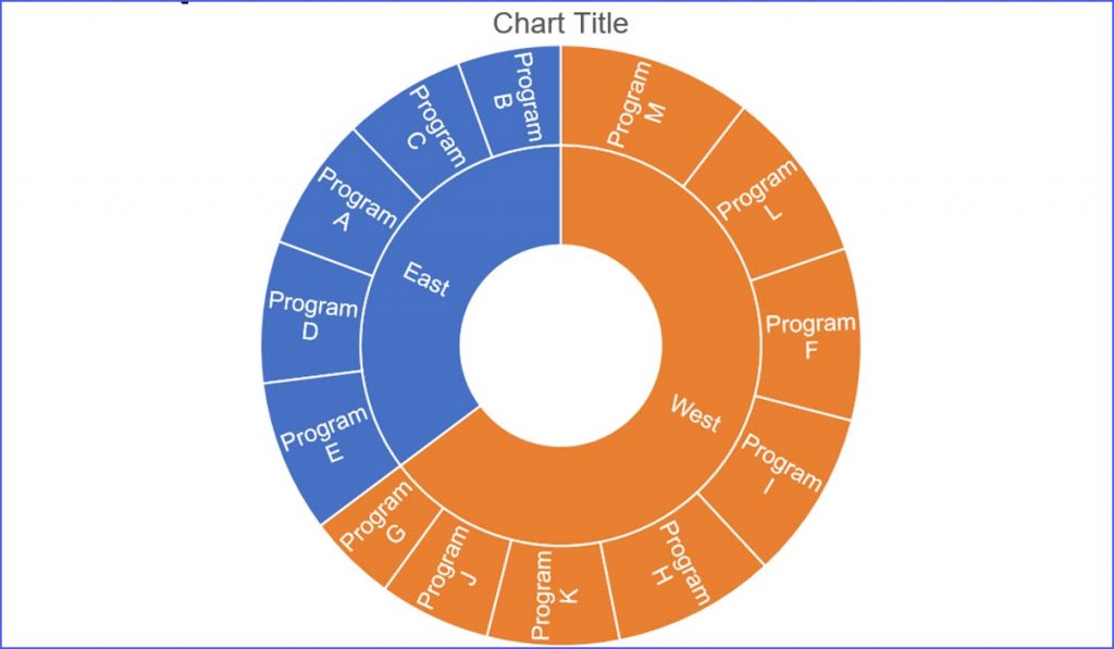
How to Make a Sunburst Chart - ExcelNotes

How to create Custom Data Labels in Excel Charts - Efficiency 365 Add default data labels Click on each unwanted label (using slow double click) and delete it Select each item where you want the custom label one at a time Press F2 to move focus to the Formula editing box Type the equal to sign Now click on the cell which contains the appropriate label Press ENTER That's it.

Multiple bar charts on one axis in excel - Super User

How to Create Mailing Labels in Word from an Excel List Step Two: Set Up Labels in Word. Open up a blank Word document. Next, head over to the "Mailings" tab and select "Start Mail Merge.". In the drop-down menu that appears, select "Labels.". The "Label Options" window will appear. Here, you can select your label brand and product number. Once finished, click "OK.".

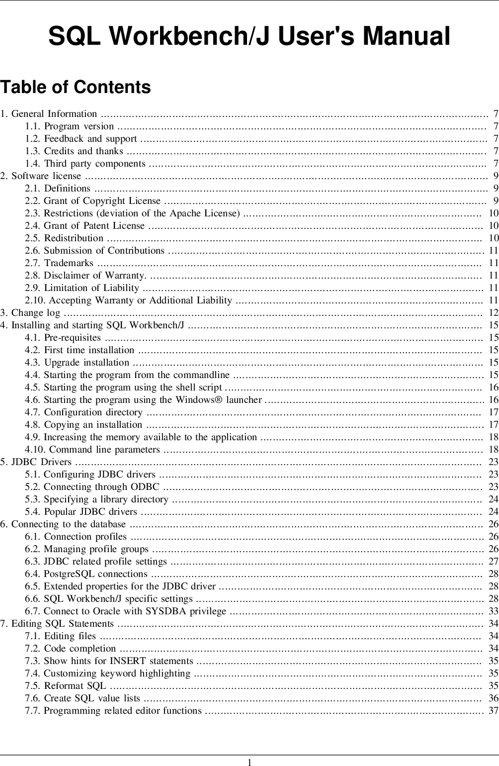
SQL Workbench/J User's Manual SQLWorkbench

Multiple Series in One Excel Chart - Peltier Tech Select Series Data: Right click the chart and choose Select Data from the pop-up menu, or click Select Data on the ribbon. As before, click Add, and the Edit Series dialog pops up. There are spaces for series name and Y values. Fill in entries for series name and Y values, and the chart shows two series.

microsoft excel - Adding data label only to the last value - Super User

How to Use Cell Values for Excel Chart Labels - How-To Geek Select the chart, choose the "Chart Elements" option, click the "Data Labels" arrow, and then "More Options.". Uncheck the "Value" box and check the "Value From Cells" box. Select cells C2:C6 to use for the data label range and then click the "OK" button. The values from these cells are now used for the chart data labels.

Microsoft Tips with Temo!: How to Add Data Labels to an Excel 2010 Chart

How to group (two-level) axis labels in a chart in Excel? - ExtendOffice (1) In Excel 2007 and 2010, clicking the PivotTable > PivotChart in the Tables group on the Insert Tab; (2) In Excel 2013, clicking the Pivot Chart > Pivot Chart in the Charts group on the Insert tab. 2. In the opening dialog box, check the Existing worksheet option, and then select a cell in current worksheet, and click the OK button. 3.

Quick Tip: Excel 2013 offers flexible data labels - TechRepublic

Multiple data labels (in separate locations on chart) Re: Multiple data labels (in separate locations on chart) You can do it in a single chart. Create the chart so it has 2 columns of data. At first only the 1 column of data will be displayed. Move that series to the secondary axis. You can now apply different data labels to each series. Attached Files 819208.xlsx‎ (13.8 KB, 265 views) Download